Microsoft Word - Protocol Development Session 5 Handout

Protocol Development Workshop

Warren Capell, MD

Session 5 – Data Analysis Plan

Session 5: Data Analysis Plan

I. Introduction

Like developing and writing protocols, data analysis is another scientific function that is assumed you can perform

because you have trained or worked in science/medicine. You might have received some basic lectures in

Epidemiology or Statistics. You might be familiar with a software program that has statistical functions. You

might have worked on a previous study where you did a relatively complex analysis, and you will “simply do this

one like last time.” This limited exposure is very different than possessing advanced knowledge of how to

approach an analysis plan for a research project. You might know enough to perform a crude analysis, but the

analysis might leave you open to criticism when you go to publish, or worse, it might lead to inaccurate results

from a flawed approach.

Take-home point: To do truly sound research, you need to have, or have access to, advanced statistical

knowledge. Even if you think you know how to analyze a data set, it is best to at least consult with a

biostatistician to make sure your approach is correct.

This need creates a problem on our campus; there simply is not enough statistical expertise available for everyone

to have access to sufficient statistical expertise. Statistical resources on campus are largely decentralized and

provided by each Department/Division. There is a central biostatistics resource within the CCTSI that can be

accessed for limited service. See section IV for brief orientation on finding help.

Because of the limitation of statistical resources, your basic strategy in developing your protocol should be as

follows:

1) Try to find expert biostatistics help by working through the resources discussed in section IV.

2) After exercising these options listed in section IV, you should have a good idea of how to construct your

study and how it will be analyzed. If you have exhausted these options and are still not exactly sure of how

your data should be analyzed, you are in a difficult position. Your science cannot go forward without some

basic understanding of how your data will be analyzed. A protocol cannot be approved without a reasoned

data analysis plan. My recommendation is that you:

a. Write a reasoned statistical analysis plan for your protocol (see section II) to move the protocol

forward and be able to start your research.

b. Over the time it takes to get your research approved and collect the data, continue to work on finding

professional help. Talk to your Division Head to see if the Division can help fund access to a

statistician. Using this approach, however, it is difficult to go back and modify your study design if it

becomes apparent that statistical input could have helped tweak the design to be more accurate or

less biased.

II. Reasoned Statistical Analysis Plan

If you’re reading this section, it means that you were unable to get professional help and you are trying to move

your protocol forward while you continue to work on finding resources. This is also a good place to start reading

if you are preparing to meet with a statistician, as it can give you a reasoned starting point to begin a discussion

of your protocol. If you have help, or if you have your own advanced knowledge of statistics, skip ahead to

section III, which discusses what should be addressed in your protocol’s Data Analysis section.

Protocol Development Workshop

Warren Capell, MD

Session 5 – Data Analysis Plan

It is important that your protocol communicate an appropriate statistical approach to analyze your outcomes. In

reviewing your data analysis plan, the IRB needs to know that there is a plan that will provide some kind of valid

generalizable knowledge (the main benefit of most research studies). An expert analysis plan is always preferred

and communicates that this study is well-positioned to meet its goals; however, even a rudimentary analysis plan

can be sufficient to meet this generalizable knowledge standard. Unfortunately, many protocols are submitted

with analysis plans that are either nonsensical, or communicate ignorance toward how to begin analyzing the

project. This section is intended to help you talk intelligently about your data structure and communicate the

broad type(s) of statistical tests you will employ.

A. Descriptive Statistics

If the purpose of your project is only to describe a phenomenon or condition you are measuring (e.g.,

number of positive tests, distribution of head circumference, prevalence of trait X, percentage of patients

responding to a single treatment), you will be using “descriptive statistics.” Descriptive statistics include

counts, percentages, means, medians, modes, proportions, standard deviations, variances, frequencies, and

histograms, among others. The key is that there are no comparisons being made between different

measures in the study; the purpose is to report the measures only. In this case, your plan can be stated as

(for example) “We will use descriptive statistics to report on the median survival in X malignancy.” Perhaps

part of your study purpose is to describe; the plan for that portion of the study will then utilize descriptive

statistics.

If the goal of your study is to make comparisons (i.e., test hypotheses), descriptive statistics are not

sufficient. Proceed to section II,B.

B. Hypothesis Testing: recognize your variables

If the goal of your study is to make comparisons between groups, arms, or conditions, you will need to

choose appropriate statistical tests of your hypotheses. To choose tests appropriately, you need to

understand your data structure. Data structure depends on the types of variables by which your predictor

conditions and outcome conditions are measured.

i. Categorical variables. Categorical variables are categories that each subject or measurement is

assigned. Categorical variables do not have any intrinsic numeric value; they are essentially labels.

Examples include color (red, blue, yellow, etc.), treatment arm (placebo, low-dose drug, high dose drug,

etc.), presence of condition (e.g., yes/no, or positive/negative), vital status (dead or alive), diagnosis

(schizophrenia, major depression, delirium, etc.). Note that since categorical variables are not numeric,

they do not have a mean, median, or distribution/variance. Either the subject meets the category or

s/he does not. Typically, counts (or proportions) of subjects in the sample that fit each category make

up the study results.

ii. Interval variables. Interval variables have an inherent numerical value. When measured, each subject

will have a particular numerical value. The numerical scale for the variable is such that the difference

between any two numbers on the scale is a constant difference (i.e., the difference between 2 and 5, is

the same as between 102 and 105). Because of their numeric value, a mean, median, and variance for

the study sample (or study arm) can be calculated once each subject’s result is measured. Interval

Protocol Development Workshop

Warren Capell, MD

Session 5 – Data Analysis Plan

variables can be further divided into Continuous (infinite number of values between any two values) and

Discrete variables (Finite number of values between any two values). For practical purposes, all interval

variables (continuous or discrete) can be lumped together for the purposes of reasoning an analysis

plan. Examples of interval variables include age, blood pressure, serum cholesterol,

a. Continuous variables. On the measurable scale for the variable, there are infinite possible values.

iii. Ordinal variables. Ordinal variables are most like categorical variables, but have a natural order to

them. They are not interval variables, however, because the difference between any two values is not a

constant difference. For example, a rating scale of Strongly agree, Agree, Neutral, Disagree, and

Strongly disagree is ordinal; there is a natural value order to the scale, but it is not possible to say that

the difference between ‘Strongly agree’ and ‘Agree’ is the same as the difference between ‘Agree’ and

‘Neutral.’ Similarly, a pain scale (0-10) is ordinal; it is not possible to say that the difference in pain

between a ‘1’ and ‘2’ is the same as the difference between ‘9’ and ’10.’ Cancer stages are another

example of an ordinal variable. Likert scales are generally ordinal. Statistically, ordinal variables can

undergo statistical testing that more closely resembles interval data (though not all of the same tests).

C. Hypothesis Testing: determine your data structure and selecting statistical tests

Thinking about your data structure is extremely helpful in determining what types of statistical tests can be

used to test your hypotheses. The best way to think about data structure is to draw a schematic of what

your data will look like when you have completed data collection. For this exercise, you will identify the

independent (or predictor) variables and the dependent (outcome) variables.

Disclaimer: This section is a rudimentary guide only. It can be helpful to zero in on the general family of

statistical tests that can be used in different situations. This discussion is not meant to replace professional

statistical advice. The application of these tests are not always appropriate because each test has underlying

assumptions that must be met. When the particular assumptions are not met, there is usually an alternate

test that should be used instead. Therefore, remember the importance of a statistical consult.

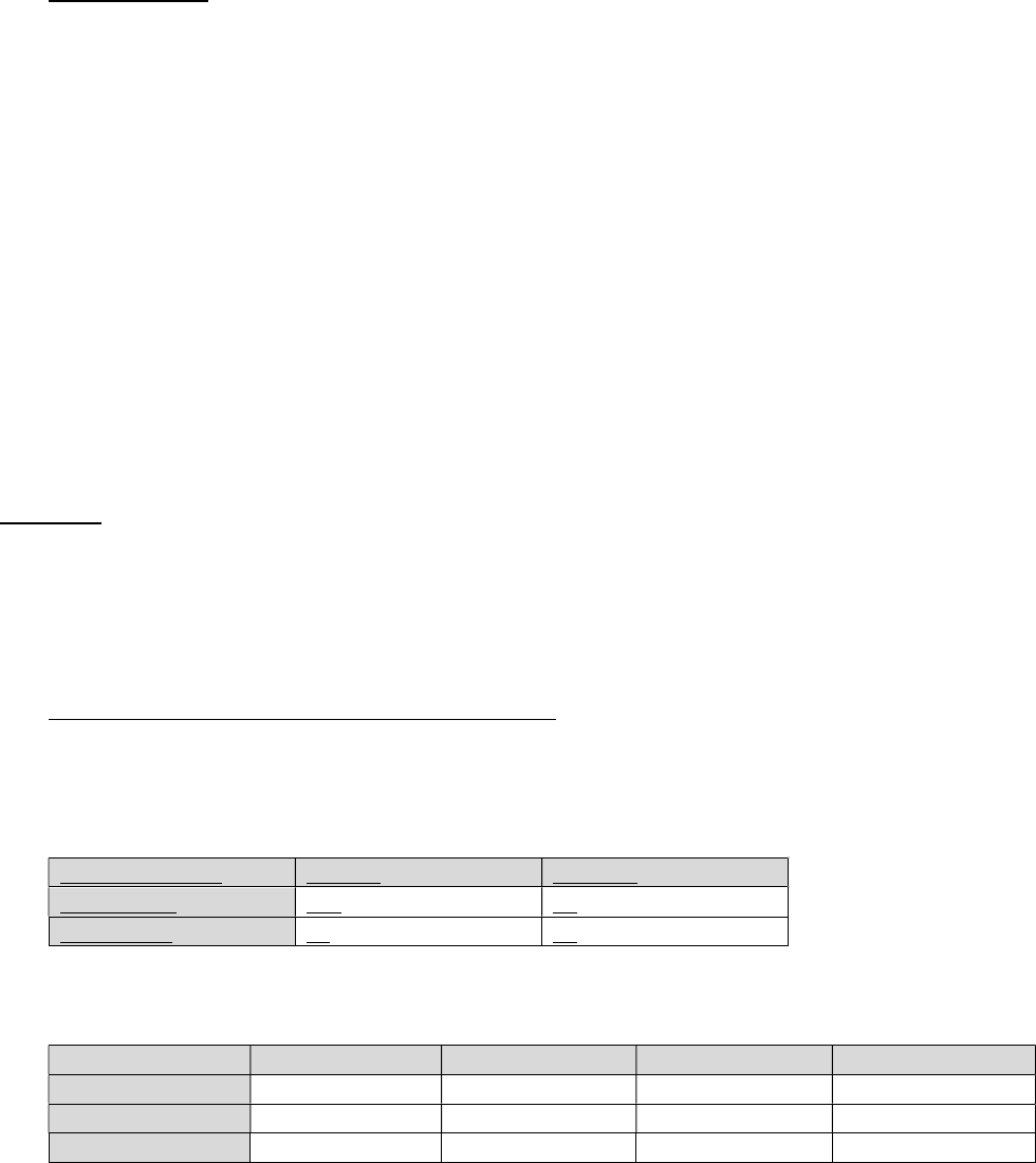
i. Independent and Dependent variables are categorical. When both independent (predictor) and

dependent (outcome) variables are categorical, it is not possible to graph the results, because there are

no numeric data; the data structure becomes an x by y table, where x is the number of independent

variable values and y is the number of dependent variable values. Take this example of data examining

pre-test clinical diagnosis and the result of a confirmatory test (2 by 2 table).

Clinical Diagnosis

Positive

Negative

Clinical

Yes

118

Clinical

Tables can be any number of x by y.

Treatment

Cells lysed

Cells injured

Cells swollen

Cells unchanged

12%

22%

41%

23%

32%

36%

15%

17%

44%

31%

20%

Protocol Development Workshop

Warren Capell, MD

Session 5 – Data Analysis Plan

The statistical test of choice for this data structure is χ

. The chi-square test examines the probability

that the distributions of observations across cells occurred by chance.

ii. Independent variable is categorical and Dependent variable is interval. A typical graph of this data

structure would look like this:

The test of choice for this data structure, when there are two independent variable values, is the two-

sample t-test.

When there is more than one independent variable value, the data structure would look like this:

The test of choice for this data structure, when there are more than two independent variable values, is

analysis of variance (ANOVA).

iii. Independent variable is time and Dependent variable is interval and measured at different time

intervals. A typical graph of this data structure would look like this:

Protocol Development Workshop

Warren Capell, MD

Session 5 – Data Analysis Plan

The test of choice for this data structure is Repeated Measures ANOVA (RMANOVA). RMANOVA

compares both the difference in values and shape of the curves (condition and time interaction).

Subsequent follow-up testing can identify specific time points that differ between groups. Sometimes,

the data presented will have this structure, but the primary outcome will be a comparison of only one

time point; in such a case, a t-test (when there are two groups compared) or ANOVA (when there are

more than two groups compared) would be the primary hypothesis test.

iv. Independent variable is time and Dependent variable is event-free status. This would be the structure

for a “time to X” analysis, such as “time to failure” or “event-free survival.” A typical graph of this data

structure would look like this:

This type of graph is known as a Kaplan-Meier plot, showing a stepwise decline over time in the number

of subjects in each group that remain free of the outcome of interest. The statistical test of choice for

this data structure is the Kaplan-Meier estimator.

v. Independent and Dependent variables are interval. A typical graph of this data structure would look like

this:

The test of choice for this data structure is the Pearson correlation coefficient, which indicates how

closely the individual points cling to a common line, and whether the variables co-vary in the same

direction or in opposite directions. Linear regression can also be performed to create a mathematical

relationship (slope) of the best-fit line.

Protocol Development Workshop

Warren Capell, MD

Session 5 – Data Analysis Plan

vi. Modeling. Some projects seek to understand how several predictor variables, put together, correlate

with a specific outcome. This type of complex analysis requires examining correlations of each variable

to see which have a general propensity to drive the outcome variable, and then performing step-wise

analyses to understand which variables independently associate with the outcome and their relative

impact. A statistician is highly advisable for any type of modeling analysis unless you are trained in this

method.

III. Writing the Data Analysis Section of the Protocol

IRBs have two primary concerns when reviewing data analysis sections: 1) That there is sound methodology for

data analysis such that generalizable knowledge will be produced by the results, and 2) that the requested

sample size for the study is justified.

A. Methodology will produce generalizable knowledge

Recall that the IRB must determine that the benefits of the research outweigh the risks. The benefit side of

this equation rests mainly with the resulting generalizable knowledge that will ultimately benefit society. If

the study has an inappropriate or flawed analysis plan that is unlikely to contribute generalizable knowledge,

the IRB cannot approve the study. Therefore, the analysis plan needs to be reasoned and a logical approach

to analyzing the data structure for the particular study. It is rare to encounter a statistician reviewer on the

IRB, but many IRB members have extensive knowledge and experience in data analysis. However, the

threshold to be approvable for an IRB may not be as high as for a scientific review committee; remember

that your protocol may also require review by a designated scientific review committee. Therefore,

obtaining expert statistical input is extremely valuable.

B. Sample size is adequately justified

Every subject that is enrolled in your study will experience some amount of risk. In order to minimize the

risks of the research (one of the IRB approval criteria) then, it is imperative that the study enroll the

minimum number of subjects necessary to answer the research question. How does one know the minimum

number of subjects required? That estimate is accomplished through a power analysis. Power analysis

informs that given the known variability in the outcome measure in the population being studied, along with

the proposed difference between the populations being measured, the number of subjects needed to fix

type 1 and type 2 error rates. The greater the variability in your outcome measure and the smaller the

proposed difference between populations, the greater the sample size must be to reliably answer the

research question.

The lack of any power analysis or justification of the requested sample size is a common problem seen at the

IRB. Additionally, sometimes studies are clearly requesting a sample size that is too small to definitively

answer the research question, yet the protocol is written as if the question will be answered with the current

study. Your study should be clear whether it is attempting to answer the research question; if so, there

should be a power analysis to demonstrate the statistical validity of the sample size. However, it is important

to realize that your study does not need to be able to definitively answer the research question.

“Generalizable knowledge” is a subjective term and does not need to represent a definitive study. Pilot

studies and feasibility studies are examples of research that is not definitive. They can expose a small

Protocol Development Workshop

Warren Capell, MD

Session 5 – Data Analysis Plan

number of subjects to risk in order to see if it is feasible or worthwhile exposing a large number of subjects to

risk in a definitive study. They can provide preliminary data to support a grant for funding a larger study.

They can lay the groundwork for the methods of a larger, definitive study. This is perfectly acceptable, but

you must acknowledge this limited goal in your study aims. If you do not clearly indicate your study is a pilot

study, you will likely be required to justify your requested sample size. If you are clear that your study is a

pilot, then you can simply explain why you have chosen the number of subjects requested; that could be for

budget reasons, but still must be adequate to achieve the stated aims of your study (e.g., to provide

preliminary data for a grant).

Performing a power analysis, again, may require the help of a statistician. There are some statistical

software packages that have power calculators. For most power analyses, you will need: 1) Some sort of

estimate of the variability of your outcome measure (from your own preliminary data or from the literature),

and 2) your assessment of what a meaningful difference would be between groups in your chosen primary

outcome measure. A quick local power calculator can be found on the College of Nursing website:

http://www.ucdenver.edu/academics/colleges/nursing/research/center-for-nursing-

research/Pages/virtualcnr.aspx

IV. Biostatistics resources

1) Talk with your mentor or Division Head to see what local resources are available to you. This is your best

chance of finding a reliable partnership for your study.

2) If not available, lobby your Division Head for this shared resource for your section; many divisions have

invested in this resource, knowing its importance for excellent science.

3) If your Division cannot provide assistance, contact the Colorado Biostatistics Consortium (cbc.ucdenver.edu).

This is the primary centralized resource on campus that can put you in touch with statistical consultations or

assistance.

4) Biostatistics program is offered by the institution through the CCTSI:

http://www.ucdenver.edu/research/CCTSI/programs-services/berd/Pages/default.aspx

5) The College of Nursing has some great on-line resources in addition to the power calculator. Performing tests

to evaluate predictive or diagnostic methods is a common theme in this workshop; the following link has some

helpful tools for this (see under the Developing and Evaluating Instruments tab):

http://www.ucdenver.edu/academics/colleges/nursing/research/center-for-nursing-

research/Pages/cnrtoolsandresources.aspx

6) Statistical software.

a. STATA: This is a preferred product because of its ease of use, point-and-click design, relative

affordability ($200-400), and plentiful online tutorials. It represents a relatively small time investment

to learn (compared to SPSS or SAS), and can pay dividends after you put in the initial time.

b. JMP: A clickable version of SAS, and it is free from the institution.

c. R: Free and widely used by statisticians, but steeper learning curve.

d. SAS: The gold standard, but quite a steep learning curve to use it.

e. Do not use Excel for statistical analysis. It is believed by many to provide inaccurate results in various

situations.